This time, we would like to use a Markov Decision Process in order to model the possibility that some actions have an uncertain effect on the agent and the environment. In particular, we will consider the scenario where at each time step the agent gets stuck in the current city with some probability.
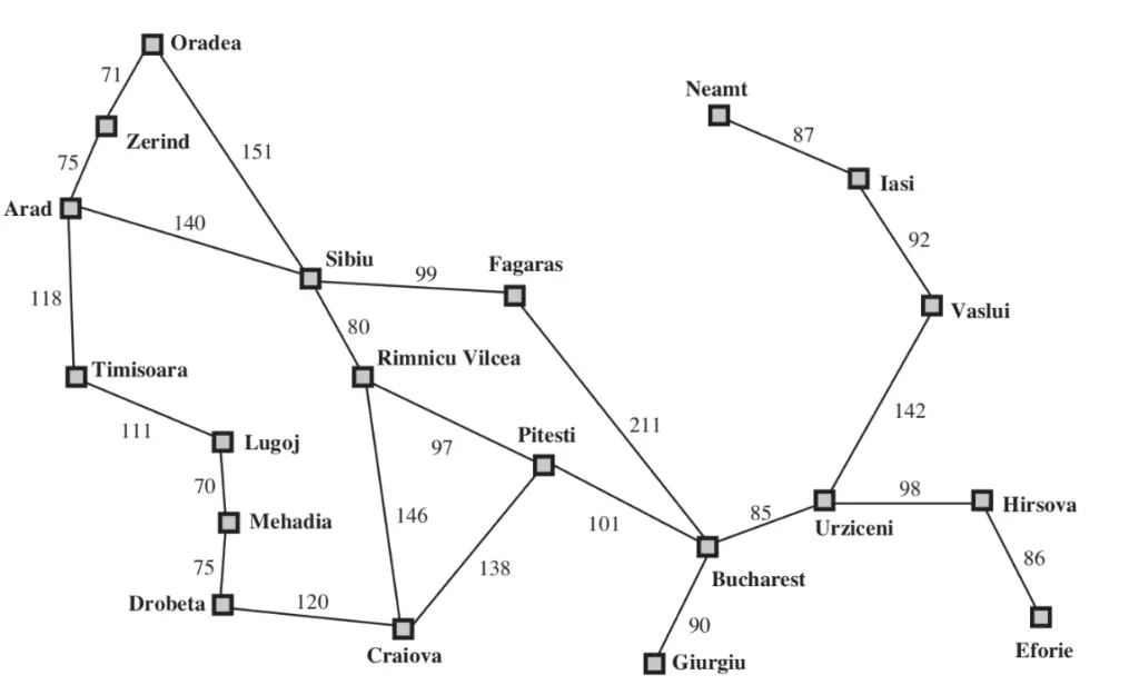
For simplicity of implementation, we will consider that for each time step $t$ of the MDP the associate state variable $S_t$ always has the same domain $D$ consisting of all 20 cities on the map.
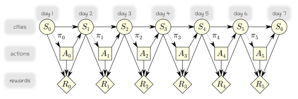
$$ S_0,S_1,\dots,S_{T-1} \in D \qquad D = \{\text{Arad},\text{Urziceni},\dots \} $$Furthermore, we will consider that from every state and value of that state, we always have the opportunity take action to move to any city, regardless of the road connectivity, i.e. $A_0,A_1,\dots,A_{T-2} \in D$. To eliminate solutions that do not respect the road constraints, we incorporate penalties in reward nodes $R_{1}, R_{2}, \dots$. Specifically, we generate a strongly negative reward if such illegal actions are chosen. As a result, the inference algorithm will effectively discard such actions. The corresponding MDP is illustrated below.
cities   = utils.cities
nbcities = len(cities)
(a) Building Probability and Reward Arrays
As a first step, we would like to build arrays of probability and reward values which will support our inferences. We will build three arrays for that purpose:
A numpy array
Pof size $N \times N \times N$ where $N$ is the number of cities, and where the first dimensions represents the current state, the second dimension represents the action being taken, and the third dimension represents the state in the next time step. The array should be built in a way that one arrives in the intended city (specified by our action) with a probability of 0.8 and stay stuck in the current city with probability 0.2. Because the process is time-independent, we need only one such matrix.A numpy array
Rmidof size $N \times N \times N$ representing the rewards at each time step. It includes an artificial negative reward of $-99$ for actions that are not allowed from the current state. It further adds a negative reward of $-1$ for transitions between two distinct cities in order to model the cost of fuel. Like for the matrixP, the first dimension represents the state, the second dimension represents the action, and the last dimension represents the state we transition to.A numpy array
Rlastof size $1 \times 1 \times N$ that adds to the reward in the last time step a reward if the goal has been achieved. Specifically, it adds a reward of $20$ if the agent arrives in Urziceni in the final step (our goal), $10$ if it terminates instead in Craiova (a fallback objective), and a reward of $0$ otherwise.
In other words, the rewards $R_0,\dots,R_4$ are given by Rmid and the reward $R_5$ is given by the sum of Rmid and Rlast.
I = numpy.eye(len(utils.cities))
Illegal = (1-I-utils.A)
print(Illegal)

def buildArrays():
    N = len(utils.cities)

    I = np.eye(N)

    Illegal = 1 - I - utils.A

    Rmid = (-99 * Illegal)[:, :, na] - 1 * utils.A[:, na, :]

    Rlast = (
        20 * I[utils.cities.index('U')] +
        10 * I[utils.cities.index('C')]
    )[na, na, :]

    P = np.zeros((N, N, N))

    for s in range(N):
        for a in range(N):
            P[s, a, s] = 0.2

            P[s, a, a] += 0.8

    return P, Rmid, Rlast
[[0. 1. 1. 1. 1. 1. 1. 1. 1. 1. 1. 1. 1. 1. 1. 0. 0. 1. 1. 0.]
 [1. 0. 1. 1. 1. 0. 0. 1. 1. 1. 1. 1. 1. 0. 1. 1. 1. 0. 1. 1.]
 [1. 1. 0. 0. 1. 1. 1. 1. 1. 1. 1. 1. 1. 0. 0. 1. 1. 1. 1. 1.]
 [1. 1. 0. 0. 1. 1. 1. 1. 1. 1. 0. 1. 1. 1. 1. 1. 1. 1. 1. 1.]
 [1. 1. 1. 1. 0. 1. 1. 0. 1. 1. 1. 1. 1. 1. 1. 1. 1. 1. 1. 1.]
 [1. 0. 1. 1. 1. 0. 1. 1. 1. 1. 1. 1. 1. 1. 1. 0. 1. 1. 1. 1.]
 [1. 0. 1. 1. 1. 1. 0. 1. 1. 1. 1. 1. 1. 1. 1. 1. 1. 1. 1. 1.]
 [1. 1. 1. 1. 0. 1. 1. 0. 1. 1. 1. 1. 1. 1. 1. 1. 1. 0. 1. 1.]
 [1. 1. 1. 1. 1. 1. 1. 1. 0. 1. 1. 0. 1. 1. 1. 1. 1. 1. 0. 1.]
 [1. 1. 1. 1. 1. 1. 1. 1. 1. 0. 0. 1. 1. 1. 1. 1. 0. 1. 1. 1.]
 [1. 1. 1. 0. 1. 1. 1. 1. 1. 0. 0. 1. 1. 1. 1. 1. 1. 1. 1. 1.]
 [1. 1. 1. 1. 1. 1. 1. 1. 0. 1. 1. 0. 1. 1. 1. 1. 1. 1. 1. 1.]
 [1. 1. 1. 1. 1. 1. 1. 1. 1. 1. 1. 1. 0. 1. 1. 0. 1. 1. 1. 0.]
 [1. 0. 0. 1. 1. 1. 1. 1. 1. 1. 1. 1. 1. 0. 0. 1. 1. 1. 1. 1.]
 [1. 1. 0. 1. 1. 1. 1. 1. 1. 1. 1. 1. 1. 0. 0. 0. 1. 1. 1. 1.]
 [0. 1. 1. 1. 1. 0. 1. 1. 1. 1. 1. 1. 0. 1. 0. 0. 1. 1. 1. 1.]
 [0. 1. 1. 1. 1. 1. 1. 1. 1. 0. 1. 1. 1. 1. 1. 1. 0. 1. 1. 1.]
 [1. 0. 1. 1. 1. 1. 1. 0. 1. 1. 1. 1. 1. 1. 1. 1. 1. 0. 0. 1.]
 [1. 1. 1. 1. 1. 1. 1. 1. 0. 1. 1. 1. 1. 1. 1. 1. 1. 0. 0. 1.]
 [0. 1. 1. 1. 1. 1. 1. 1. 1. 1. 1. 1. 0. 1. 1. 1. 1. 1. 1. 0.]]
WE can test the implementation using the following code.
P,Rmid,Rlast = buildArrays()

print(P[:1,:2,:])
print(Rmid[0,-2:,:])
print(Rlast[:,:,:])
[[[1.  0.  0.  0.  0.  0.  0.  0.  0.  0.  0.  0.  0.  0.  0.  0.  0.
   0.  0.  0. ]
  [0.2 0.8 0.  0.  0.  0.  0.  0.  0.  0.  0.  0.  0.  0.  0.  0.  0.
   0.  0.  0. ]]]
[[ -99.  -99.  -99.  -99.  -99.  -99.  -99.  -99.  -99.  -99.  -99.  -99.
   -99.  -99.  -99. -100. -100.  -99.  -99. -100.]
 [  -0.   -0.   -0.   -0.   -0.   -0.   -0.   -0.   -0.   -0.   -0.   -0.
    -0.   -0.   -0.   -1.   -1.   -0.   -0.   -1.]]
[[[ 0.  0. 10.  0.  0.  0.  0.  0.  0.  0.  0.  0.  0.  0.  0.  0.  0.
   20.  0.  0.]]]
(b) Value Iteration and Expected Utilities under Rational Acting
Now, we can carry out the value iteration algorithm. This will enables us to measure what is the expected utility if being in Urziceni on the first day and acting rationally. The recursive equations for generating the expected utilities when following an optimal policy are given by: \begin{align*} Q(A_t,S_t) &= \sum_{S_{t+1} \in D} \big[R(S_t,A_t,S_{t+1}) + U(S_{t+1})\big] P(S_{t+1}|A_t,S_t)\\ U(S_t) &= \max_{A_t \in D} Q(A_t,S_t) \end{align*} One first sets $U(S_6)$ to an empty array, and then compute $U(S_5),U(S_4),\dots$ by repeated application of this equation. This can be implemented compactly as:
U = numpy.zeros([len(utils.cities)])

for t in [5,4,3,2,1,0]:
    R = Rmid + (Rlast if t==5 else 0)
    Q = (P*(U+R)).sum(axis=-1)
    U = Q.max(axis=-1)

utils.printvalues(U)
           Arad: 14.335
      Bucharest: 18.999
        Craiova: 16.739
        Dobreta: 14.699
         Eforie: 17.970
        Fagaras: 17.970
        Giurgiu: 17.970
        Hirsova: 18.999
           Iasi: 17.970
          Lugoj: 7.593
        Mehadia: 11.279
          Neamt: 16.686
         Oradea: 14.335
        Pitesti: 17.972
 Rimnicu Vilcea: 16.737
          Sibiu: 16.694
      Timisoara: 9.692
       Urziceni: 20.000
         Vaslui: 18.999
         Zerind: 9.692
and the resulting utilities $U(S_0)$ can then be printed. This correspond to the expected utility one would get if starting in each city on the map and acting rationally. As can be observed, our utility associated to starting in Arad is around 14. If we would have started in a different city, e.g. closer to Urziceni, the expected utility would increase, with the maximum utility obtained if being already in Urziceni on day 1.
(c) Extracting the Policy
We now would like to determine what policy is required at each time step in order to achieve the desired high expected utility. Implement an extension of the value iteration procedure above that keeps track this time of the best actions at each time step. As a reminder, the best actions can be extracted using the equation:
\begin{align*} \pi_t(S_t) &= \arg\max_{A_t \in D} Q(A_t,S_t) \end{align*}this function return a matrix $A$ of size $6 \times \#\,\text{cities}$ indicating, for any time step and state value (city) at that time step, the best possible action to be taken.
def getPolicy():
    P, Rmid, Rlast = buildArrays()
    U = np.zeros(len(utils.cities))
    A = np.zeros((6, len(utils.cities)), dtype=int)

    for t in [5, 4, 3, 2, 1, 0]:
        R = Rmid + (Rlast if t == 5 else 0)

        Q = (P * (U + R)).sum(axis=-1)
        A[t] = Q.argmax(axis=-1)
        U = Q.max(axis=-1)

    return A
The policy is visualized by running the code below.
utils.printpolicy(getPolicy())
day 1  | day 2  | day 3  | day 4  | day 5  | day 6
A -> S | A -> S | A -> S | A -> S | A -> A | A -> A
B -> U | B -> U | B -> U | B -> U | B -> U | B -> U
C -> P | C -> P | C -> P | C -> P | C -> C | C -> C
D -> C | D -> C | D -> C | D -> C | D -> C | D -> C
E -> H | E -> H | E -> H | E -> H | E -> H | E -> E
F -> B | F -> B | F -> B | F -> B | F -> B | F -> F
G -> B | G -> B | G -> B | G -> B | G -> B | G -> G
H -> U | H -> U | H -> U | H -> U | H -> U | H -> U
I -> V | I -> V | I -> V | I -> V | I -> V | I -> I
L -> M | L -> M | L -> M | L -> M | L -> L | L -> L
M -> D | M -> D | M -> D | M -> D | M -> D | M -> M
N -> I | N -> I | N -> I | N -> I | N -> N | N -> N
O -> S | O -> S | O -> S | O -> S | O -> O | O -> O
P -> B | P -> B | P -> B | P -> B | P -> B | P -> C
R -> P | R -> P | R -> P | R -> P | R -> C | R -> C
S -> F | S -> F | S -> F | S -> F | S -> R | S -> S
T -> A | T -> A | T -> A | T -> T | T -> T | T -> T
U -> U | U -> U | U -> U | U -> U | U -> U | U -> U
V -> U | V -> U | V -> U | V -> U | V -> U | V -> U
Z -> A | Z -> A | Z -> A | Z -> Z | Z -> Z | Z -> Z
We observe that the best action if starting in Arad is to first move to Sibiu. If the action get carried out correctly, one then moves from Sibiu to Fagaras, etc. Interestingly, as time passes, reaching Urziceni may no longer be possible from certain locations. Hence the rational action may in these cases be to opt for the fallback objective of going to Craiova, or less ambitious, simply stay in the current city to avoid any further spendings on fuel.